Building a Gaussian Splatting Renderer in OpenGL

Posted Jan 4, 2025 Updated Jan 6, 2025

By Justin Stephens

19 min read

In this article, I will discuss how I built a gaussian splatting renderer using OpenGL. I want to keep it lean, concise, clear, and focus on the important bits. It’s for this reason that I won’t be diving deep into spherical harmonics nor basic OpenGL concepts such as creating a window or shader programs. I aim to make this post digestible by those who lack graphics API knowledge, but some degree of familiarity would be helpful. Additionally, I will include links and references to other pieces of text that dive further into some of the details I’ve skipped over if you are interested in learning more.

Let us first begin by discussing the dataset being used, how to load it, and the major components that are needed. The data I’ve used for my renderer has been provided by ShapeSplat. Each set of gaussians come as a .ply file. I’ve used the Point Cloud Library (PCL) to load these files.

First, we will need to create a custom structure to hold our data. This is required to load the file using PCL.

  
// Define custom point type with exact property names
struct GaussianData {
	PCL_ADD_POINT4D;                  

	float nx, ny, nz;                
	float f_dc_0, f_dc_1, f_dc_2;     
	float opacity;
	float scale_0, scale_1, scale_2;
	float rot_0, rot_1, rot_2, rot_3;

	PCL_MAKE_ALIGNED_OPERATOR_NEW 
};

  
// Register the custom point type with PCL
POINT_CLOUD_REGISTER_POINT_STRUCT(
	GaussianData,
	(float, x, x) (float, y, y) (float, z, z)
	(float, nx, nx) (float, ny, ny) (float, nz, nz)
	(float, f_dc_0, f_dc_0) (float, f_dc_1, f_dc_1) (float, f_dc_2, f_dc_2)
	(float, opacity, opacity)
	(float, scale_0, scale_0) (float, scale_1, scale_1) (float, scale_2, scale_2)
	(float, rot_0, rot_0) (float, rot_1, rot_1) (float, rot_2, rot_2) (float, rot_3, rot_3)
);

We can define a variable using our new point type to store our data.

  
// Create a PointCloud with the custom point type
pcl::PointCloud<GaussianData>::Ptr cloud(new pcl::PointCloud<GaussianData>);

To access the data:

  
// Accessing x
cloud->points[idx].x;

// Accessing scale_1
cloud->points[idx].scale_1;

// Accessing rot_3
cloud->points[idx].rot_3;

// Etc.. 

Now that we have loaded our data, there are some preprocessing steps that must be done before we can start rendering our gaussians.

First, we will normalize the rotation values to ensure the quaternion has a magnitude of 1, as required for a valid unit quaternion. This process ensures all rotations are consistent and preserves the direction of the rotation, which is the key property we are interested in.

  
glm::vec4 normalizeRotation(glm::vec4& rot) {
	float sumOfSqaures = rot.x * rot.x + rot.y * rot.y + rot.z * rot.z + rot.w * rot.w;
	float normalizedVal = std::sqrt(sumOfSqaures);
	return glm::vec4(rot.x / normalizedVal, rot.y / normalizedVal, rot.z / normalizedVal, rot.w / normalizedVal);
};

Next, we take the exponent of our scale values.

  
glm::vec3 scales = glm::exp(glm::vec3(point.scale_0, point.scale_1, point.scale_2));

For the opacity, we need to ensure it is within a range of 0 - 1. With 0 being transparent and 1 representing full opacity. To map our values to this range, we can pass them through a sigmoid function.

  
float sigmoid(float opacity) {
	return 1.0 / (1.0 + std::exp(-opacity));
};

float opacity = sigmoid(point.opacity)

Finally, we need to transform the SH values into their RGB colors. The function is simple in the case of a 0-th degree SH calculation. However, higher degrees would require more advanced calculations. The code for these higher degree calculations can be found in the original gaussian splatting repo.

  
const float C0 = 0.28209479177387814f;

glm::vec3 SH2RGB(glm::vec3& color) {
	return 0.5f + C0 * color;
};

glm::vec3 RGB = SH2RGB(glm::vec3(point.f_dc_0, point.f_dc_1, point.f_dc_2));

After completing the data processing, we store the data into a flattened 1D vector. This structure simplifies instancing, which is a technique for rendering multiple copies of an object with a single draw call. To use instancing effectively, all required data must be readily available during the draw call. While storing all data in a single vector is one approach to enable instancing, it is not the only method. An alternative approach is to organize the data into multiple separate structures. However, this single-vector approach is the method I choose for my implementation for conciseness.

  
std::vector<float> flatGaussianData;
flatGaussianData.reserve(numInstances * 14);

for (const auto& point : splatCloud->points) {
	glm::vec4 tempRots = glm::vec4(point.rot_0, point.rot_1, point.rot_2, point.rot_3);
	glm::vec4 normTempRots = normalizeRotation(tempRots);

	flatGaussianData.push_back(point.x);
	flatGaussianData.push_back(point.y);
	flatGaussianData.push_back(point.z);

	flatGaussianData.push_back(normTempRots.x);
	flatGaussianData.push_back(normTempRots.y);
	flatGaussianData.push_back(normTempRots.z);
	flatGaussianData.push_back(normTempRots.w);

	flatGaussianData.push_back(glm::exp(point.scale_0));
	flatGaussianData.push_back(glm::exp(point.scale_1));
	flatGaussianData.push_back(glm::exp(point.scale_2));

	flatGaussianData.push_back(sigmoid(point.opacity));

	flatGaussianData.push_back(SH2RGB(point.f_dc_0));
	flatGaussianData.push_back(SH2RGB(point.f_dc_1));
	flatGaussianData.push_back(SH2RGB(point.f_dc_2));
};

Now that we have all of our data, what is it actually being applied to?

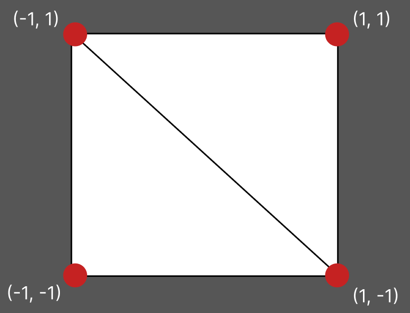
First, we need to create an object for these transformations to affect. In this case, we will create a quad as our object, which can be constructed using two triangles. Since our two triangles share certain vertices, we only need to define 4 unique vertices.

  
GLfloat quad_v[] = {
	-1.0f, 1.0f,
	1.0f, 1.0f,
	1.0f, -1.0f,
	-1.0f, -1.0f
};

GLuint quad_f[] = {
	0, 1, 2,
	0, 2, 3
};

Here we create the VAO, VBO, and EBO. These are essential components for organizing and rendering vertex data in OpenGL. The VAO stores the configuration state for our vertex data, linking to the VBO and EBO. It describes how the vertex attributes are organized and how vertex data should be indexed. The VBO stores vertex data (e.g., positions) in GPU memory, minimizing communication between the CPU and GPU. The EBO stores the indices for our vertices so we can reuse vertex data.

Next, we retrieve the location of the quadPosition attribute from the shader program and configure how the vertex data should be passed to this attribute.

  
unsigned int VAO, VBO, EBO;
// Generate VAO, VBO, & EBO
glGenVertexArrays(1, &VAO);
glGenBuffers(1, &VBO);
glGenBuffers(1, &EBO);

glBindVertexArray(VAO);

glBindBuffer(GL_ARRAY_BUFFER, VBO);
glBufferData(GL_ARRAY_BUFFER, sizeof(quad_v), quad_v, GL_STATIC_DRAW);

glBindBuffer(GL_ELEMENT_ARRAY_BUFFER, EBO);
glBufferData(GL_ELEMENT_ARRAY_BUFFER, sizeof(quad_f), quad_f, GL_STATIC_DRAW);

GLint quad_position = glGetAttribLocation(shaderProgram, "quadPosition");
glVertexAttribPointer(quad_position, 2, GL_FLOAT, GL_FALSE, 0, (void*)0);
glEnableVertexAttribArray(quad_position);

// Unbind VBO and EBO
glBindBuffer(GL_ARRAY_BUFFER, 0);
glBindBuffer(GL_ELEMENT_ARRAY_BUFFER, 0);

  
// Inside the vertex shader: 
layout (location = 0) in vec2 quadPosition; 

Going back to our gaussian data, how do we pass it into our shader to be used? We can use a Shader Storage Buffer Object (SSBO). An SSBO is advantageous when you need general-purpose, large-scale data storage accessible from shaders.

  
GLuint setupSSBO(const GLuint& bindIdx, const auto& bufferData) {
		GLuint ssbo;
		// Generate SSBO
		glGenBuffers(1, &ssbo);
		// Bind ssbo to GL_SHADER_STORAGE_BUFFER
		glBindBuffer(GL_SHADER_STORAGE_BUFFER, ssbo);
		// Populate GL_SHADER_STORAGE_BUFFER with our data
		glBufferData(GL_SHADER_STORAGE_BUFFER, bufferData.size() * sizeof(int), bufferData.data(), GL_STATIC_DRAW);
		// Specify the index of the binding (bindIdx)
		glBindBufferBase(GL_SHADER_STORAGE_BUFFER, bindIdx, ssbo);
		// Unbind ssbo to GL_SHADER_STORAGE_BUFFER
		glBindBuffer(GL_SHADER_STORAGE_BUFFER, ssbo);
	
		return ssbo;
};

GLuint pointsBindIdx = 1;
GLuint ssbo1 = setupSSBO(pointsBindIdx, flatGaussianData);

  
// In vertex shader:
layout (std430, binding=1) buffer gaussians_data {
	float gData[];
};

Take note of the bindIdx used to create the SSBO and the binding parameter in our shader.

Just like we did for the data of our gaussians, we can create an SSBO to store indices of our gaussians sorted by depth.

  
GLuint sortedBindIdx = 2;
GLuint ssbo2 = setupSSBO(sortedBindIdx, gausIdx);

  
// In vertex shader:
layout (std430, binding=2) buffer gaussians_order {
	int sortedGaussianIdx[];
};

Here we define a function that sorts our gaussians based on their depth. This depth is calculated using our view matrix. Once we have the depth for each gaussian, we pair it with the gaussian’s original index and sort these pairs by their depth. Finally, we extract the sorted indices, which is used to access the points in back-to-front order so we can perform alpha blending.

  
std::vector<int> sortGaussians(const auto& splatCloud, const glm::mat3& viewMat) {
	std::vector<std::pair<float, int>> depthIndex;
	size_t count = 0;
	for (const auto& point : splatCloud->points) {

		const glm::vec3 xyz = glm::vec3(point.x, point.y, point.z);
		glm::vec3 xyzView = viewMat * xyz;

		float depth = xyzView.z;

		depthIndex.emplace_back(depth, static_cast<int>(count));
		++count;
	}

	std::sort(depthIndex.begin(), depthIndex.end(), [](const std::pair<float, int>& a, const std::pair<float, int>& b) {
		return a.first < b.first;
		});

	std::vector<int> sortedIndices;
	sortedIndices.reserve(depthIndex.size());
	for (const auto& pair : depthIndex) {
		sortedIndices.push_back(pair.second);
	}
	return sortedIndices;
};

gausIdx = sortGaussians(cloud, glm::mat3(viewMat));

To accurately perform alpha blending, we need to enable blending in OpenGL and set our blending equation

  
	glEnable(GL_BLEND);
	glBlendFunc(GL_SRC_ALPHA, GL_ONE_MINUS_SRC_ALPHA);

Here we create the view and projection matrices. The view matrix transforms 3D world coordinates into view space (AKA camera space). This transformation orients the scene relative to the camera. The projection matrix transforms the 3D view space coordinates into clip space and applies perspective distortion to mimic how we perceive depth in the real world. In clip space, objects outside the camera’s frustum (field of view) are clipped.

GLM provides a function for creating a perspective projection matrix using four primary parameters: the field of view (FOV) in radians, the aspect ratio (width divided by height), the znear (distance to the near clipping plane), and the zfar (distance to the far clipping plane). These parameters define the camera’s view frustum, which determines how 3D objects are projected onto the 2D screen.

  
float fov = 90.0f;
float znear = 0.01f;
float zfar = 100.f

// Inside main render loop:
glm::mat4 projection = glm::mat4(1.0f);

// Create projection matrix
projection = glm::perspective(glm::radians(fov), (float)SCREEN_WIDTH / (float)SCREEN_HEIGHT, znear, zfar;
// Assign projection matrix to a shader uniform called projection
unsigned int projLoc = glGetUniformLocation(shaderProgram, "projection");
glUniformMatrix4fv(projLoc, 1, GL_FALSE, glm::value_ptr(projection));

Additionally, GLM has a function that enables us to create a view matrix using the following components. The camera’s position (the origin of its coordinate system), the direction the camera is looking (often referred to as the forward vector), and the camera’s up vector, which helps compute the camera’s local coordinate system. These components are used to define the camera’s right, up, and forward axes, ensuring the camera maintains a consistent orientation and produces an appropriate transformation from world coordinates to the camera’s local space.

  
// Inside main render loop:
glm::mat4 view = glm::mat4(1.0f);

// Create view matrix
view = glm::lookAt(cameraPos, cameraPos + cameraDirection, cameraUp);
// Assign view matrix to a shader uniform called view
unsigned int viewLoc = glGetUniformLocation(shaderProgram, "view");
glUniformMatrix4fv(viewLoc, 1, GL_FALSE, glm::value_ptr(view));

Here we calculate intrinsic camera parameters to help construct our Jacobian matrix: - Htany represents the vertical extent of the normalized camera space at a unit depth. The value of htany gives the half-angle of the vertical FOV, which corresponds to the vertical extent in our camera’s normalized space. It effectively captures how far the camera can see vertically at a unit distance from the camera along the z-axis. - Htanx represents the horizontal extent of the normalized camera space at a unit depth. It is calculated by scaling htany according to the screen’s aspect ratio. The result provides the normalized horizontal extent of the camera’s view at unit depth. - Focal_z represent the focal length of the camera in terms of the screen height. It is derived from the relationship between the vertical FOV and the screen resolution. The focal length is key in mapping normalized camera space to screen space.

  
// Calculated outside render loop:
float htany = tan(glm::radians(fov) / 2);
float htanx = htany / SCREEN_HEIGHT * SCREEN_WIDTH;
float focal_z = SCREEN_HEIGHT / (2 * htany);
hfov_focal = glm::vec3(htanx, htany, focal_z);

// Inside main render loop:
glUniform3f(glGetUniformLocation(shaderProgram, "hfov_focal"), hfov_focal.x, hfov_focal.y, hfov_focal.z);

Inside the main render loop, we can bind our VAO and draw our objects using instancing.

  
// Inside main render loop: 
glBindVertexArray(VAO);
glDrawElementsInstanced(GL_TRIANGLES, 6, GL_UNSIGNED_INT, (void*)0, numInstances);
glBindVertexArray(0);

glfwSwapBuffers(window);
glfwPollEvents();

This is the beginning of our vertex shader. Recall the order of insertion when we created our vector of gaussian data. Here we define the starting positions for each piece of data and create some helper functions.

  
#version 430 core

layout (location = 0) in vec2 quadPosition; 

#define POS_IDX 0
#define ROT_IDX 3
#define SCALE_IDX 7
#define OPACITY_IDX 10
#define SH_IDX 11
#define SH_DIM 3
		
layout (std430, binding=1) buffer gaussians_order {
	int sortedGaussianIdx[];
};

layout (std430, binding=2) buffer gaussians_data {
	float gData[];
};

vec3 get_vec3(int offset) {
	return vec3(gData[offset], gData[offset + 1], gData[offset + 2]);
};

vec4 get_vec4(int offset) {
	return vec4(gData[offset], gData[offset + 1], gData[offset + 2], gData[offset+3]);
};

  
// Uniforms set previously
uniform mat4 view;
uniform mat4 projection;
uniform vec3 hfov_focal;

// Fragment shader inputs
out vec3 outColor;
out float opacity;

For every instance of our quad being rendered, we find the corresponding sorted gaussian index. We then use this value to index into our large vector of gaussian data and grab the appropriate pieces of information.

  
int quadId = sortedGaussianIdx[gl_InstanceID];
int total_dim = 3 + 4 + 3 + 1 + SH_DIM;
int start = quadId * total_dim;

vec3 center = get_vec3(start + POS_IDX);
vec3 colorVal = get_vec3(start + SH_IDX);
vec4 rotations = get_vec4(start + ROT_IDX);
vec3 scale = get_vec3(start + SCALE_IDX);

mat3 cov3d = computeCov3D(rotations, scale);

Here we compute our 3D covariance matrix which describes the shape, orientation, and spread of our gaussians in 3D space. This covariance matrix can be assembled using our rotation and scaling values. This function is similar to the function in the original gaussian splatting paper. However, I’ve split the calculation of the rotation matrix by rows, but this is only for clarity.

  
mat3 computeCov3D(vec4 rots, vec3 scales) {

  float scaleMod = 1.0f;

  vec3 firstRow = vec3(
    1.f - 2.f * (rots.z * rots.z + rots.w * rots.w),
    2.f * (rots.y * rots.z - rots.x * rots.w),      
    2.f * (rots.y * rots.w + rots.x * rots.z)       
  );

  vec3 secondRow = vec3(
    2.f * (rots.y * rots.z + rots.x * rots.w),       
    1.f - 2.f * (rots.y * rots.y + rots.w * rots.w), 
    2.f * (rots.z * rots.w - rots.x * rots.y)        
  );

  vec3 thirdRow = vec3(
    2.f * (rots.y * rots.w - rots.x * rots.z),       
    2.f * (rots.z * rots.w + rots.x * rots.y),     
    1.f - 2.f * (rots.y * rots.y + rots.z * rots.z) 
  );


  mat3 scaleMatrix = mat3(
    scaleMod * scales.x, 0, 0, 
    0, scaleMod * scales.y, 0,
    0, 0, scaleMod * scales.z
  );

  mat3 rotMatrix = mat3(
    firstRow,
    secondRow,
    thirdRow
  );

  mat3 mMatrix = scaleMatrix * rotMatrix;

  mat3 sigma = transpose(mMatrix) * mMatrix;
  return sigma;
};

Here we are applying transformations

  
// Apply view matrix to our gaussian's xyz
vec4 cam = view * vec4(center, 1.0);
// Apply projection matrix 
vec4 pos2d = projection * cam;

// Perform perspective division to project coordinates into NDC
pos2d.xyz = pos2d.xyz / pos2d.w;
pos2d.w = 1.f;

vec2 wh = 2 * hfov_focal.xy * hfov_focal.z;

// Set limits to avoid extreme perspective distortion & contrain effects of outliers
float limx = 1.3 * hfov_focal.x;
float limy = 1.3 * hfov_focal.y;

float txtz = cam.x / cam.z;
float tytz = cam.y / cam.z;

// Clamped versions of txtz and tytz 
float tx = min(limx, max(-limx, txtz)) * cam.z;
float ty = min(limy, max(-limy, tytz)) * cam.z; 

// Cull
if (any(greaterThan(abs(pos2d.xyz), vec3(1.3)))) {
	gl_Position = vec4(-100, -100, -100, 1);
	return;	
}

Projection transformations, such as perspective projection, are inherently non-linear (not affine). These transformations are spatially variable, meaning their effects — like skewing, warping, or distortion — depend on an object’s position or depth. For instance, perspective projection makes objects closer to the camera appear larger while shrinking those farther away, often discarding depth information. It is much simpler to apply a non-linear transformation to a single point because the point is a deterministic value.

In the context of Gaussian distributions, the covariance matrix encodes both the spread of the distribution along different directions (variances) and the relationships between axes (covariances). When transforming a Gaussian to a new coordinate system, its covariance matrix must be updated to reflect the new spread and orientation. However, non-linear (not affine) transformations complicate this process because their effects vary across space, unlike linear (affine) transformations which can be captured with a constant matrix. This means that non-linear transformations applied at one point in the Gaussian distribution (e.g., near the mean) will generally differ from that applied at other points (e.g., farther from the mean). These spatially varying transformations make it challenging to directly determine how the covariance matrix transforms as the Gaussian is mapped to a new coordinate system. Additionally, a non-linear transformation could potentially distort the spread of the Gaussian in complex ways, introducing relationships between axes that were not present in the original distribution.

Instead of tackling this complexity directly, we can create a local approximation by treating the transformation as linear in the immediate vicinity of the Gaussian’s mean. This is a reasonable approach because most of the distribution’s probability is concentrated around the mean. By focusing on this region we can approximate the non-linear transformation using the first order Taylor expansion (the Jacobian) which is a linear mapping.

To approximate the non-linear transformation locally, we calculate the Jacobian matrix of the transformation function at the mean of the Gaussian. In our case, the non-linear transformation function being applied is the projection transformation which maps coordinates in camera space to clip space.

For a 3D to 2D perspective projection, the Jacobian matrix has the following structure:

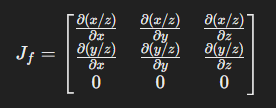
The first row represents how changes in x and y affect the new x coordinate (x’) in 2D. The second row represents how changes in x and y affect the new y coordinate (y’) in 2D. The third row is 0 because the perspective projection doesn’t affect the third coordinate.

For a perspective projection transformation, we can use intrinsic camera parameters to construct the Jacobian:

  
mat3 J = mat3(
  hfov_focal.z / cam.z, 0., -(hfov_focal.z * tx) / (cam.z * cam.z),
  0., hfov_focal.z / cam.z, -(hfov_focal.z * ty) / (cam.z * cam.z),
  0., 0., 0.
);
			
			
mat3 T = transpose(mat3(view)) * J;

mat3 cov2d = transpose(T) * transpose(cov3d) * T;

cov2d[0][0] += 0.3f;
cov2d[1][1] += 0.3f; 

if (det == 0.0f)
	gl_Position = vec4(0.f, 0.f, 0.f, 0.f);

float det_inv = 1.f / det;
conic = vec3(cov2d[1][1] * det_inv, -cov2d[0][1] * det_inv, cov2d[0][0] * det_inv);

  
// Project quad into screen space
vec2 quadwh_scr = vec2(3.f * sqrt(cov2d[0][0]), 3.f * sqrt(cov2d[1][1]));

// Convert screenspace quad to NDC
vec2 quadwh_ndc = quadwh_scr / wh * 2;

  
// Update gaussian's position w.r.t the quad in NDC
pos2d.xy = pos2d.xy + quadPosition * quadwh_ndc;

// Calculate where this quad lies in pixel coordinates 
coordxy = quadPosition * quadwh_scr;

// Set position
gl_Position = pos2d;

// Send values to fragment shader 
outColor = colorVal;
opacity = gData[start + OPACITY_IDX];

Here we are in the fragment shader. After all of our calculations, rendering the final color is fairly simple.

  
const char* fragmentShaderSource = R"(
  #version 430 core

  in vec3 outColor;
  in float opacity;
  in vec3 conic;
  in vec2 coordxy;

  out vec4 FragColor;

  void main() {			
    float power = -0.5f * (conic.x * coordxy.x * coordxy.x + conic.z * coordxy.y * coordxy.y) - conic.y * coordxy.x * coordxy.y;
    if(power > 0.0f) discard;
    float alpha = min(0.99f, opacity * exp(power));
    if(alpha < 1.f / 255.f) discard;
    FragColor = vec4(outColor, alpha);
  }
)";

And with that, you should be able to rasterize a set of 3D gaussians! This is by no means a comprehensive renderer. But, hopefully I’ve explained it well enough to help you get started or cleared up some confusion you might’ve had. If you read this and are more confused than before.. let me first apologize. Secondly, I would encourage you to check out some of these resources below. If you have any suggestions for improvements or see a mistake I made, please reach out!

References

@Article{kerbl3Dgaussians,
      author       = {Kerbl, Bernhard and Kopanas, Georgios and Leimk{\"u}hler, Thomas and Drettakis, George},
      title        = {3D Gaussian Splatting for Real-Time Radiance Field Rendering},
      journal      = {ACM Transactions on Graphics},
      number       = {4},
      volume       = {42},
      month        = {July},
      year         = {2023},
      url          = {https://repo-sam.inria.fr/fungraph/3d-gaussian-splatting/}
}

https://www.cs.umd.edu/~zwicker/publications/EWAVolumeSplatting-VIS01.pdf

https://martinoshelf.neocities.org/gaussiansplatting-in-lovr

https://www.songho.ca/opengl/gl_projectionmatrix.html

https://shi-yan.github.io/how_to_render_a_single_gaussian_splat/

https://github.com/limacv/GaussianSplattingViewer

https://github.com/cvlab-epfl/gaussian-splatting-web

https://github.com/playcanvas/supersplat

Gaussian Splatting, OpenGL

Gaussian Splatting OpenGL

This post is licensed under CC BY 4.0 by the author.

Building a Gaussian Splatting Renderer in OpenGL

References

Trending Tags